一、前言
我经常需要绘制根轨迹、Nyquist 图之类的图象,MATLAB 启动确实是有点慢,可以使用 Python 的 control 库来迅速的画出所需的图象。
下面是简单的例子。
二、画图
(一)准备工作
- 安装 control 库:
1 | pip install control |
- 导入所需要的库
下面的库都是后续操作所要使用的:
1 | import control as ctrl |
- 定义 tf2latex 函数
tf2latex 用于将传递函数转换成 LaTeX 字符串,方便后续使用。
1 | # Transfer Function 2 LaTex |
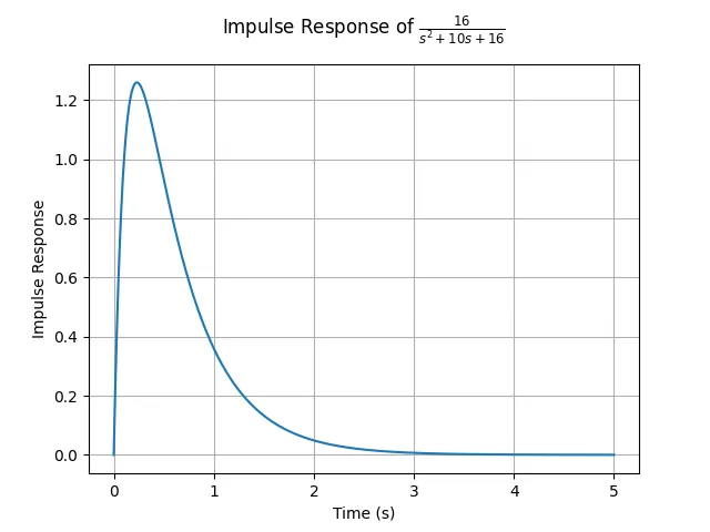
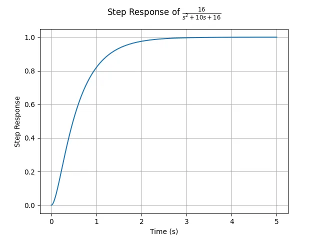
(二)系统响应
对于闭环传递函数为
- 定义绘图函数
1 | # Draw Impulse Response |
- 定义传递函数并绘图
1 | # Define Transfer Function |
- 图象
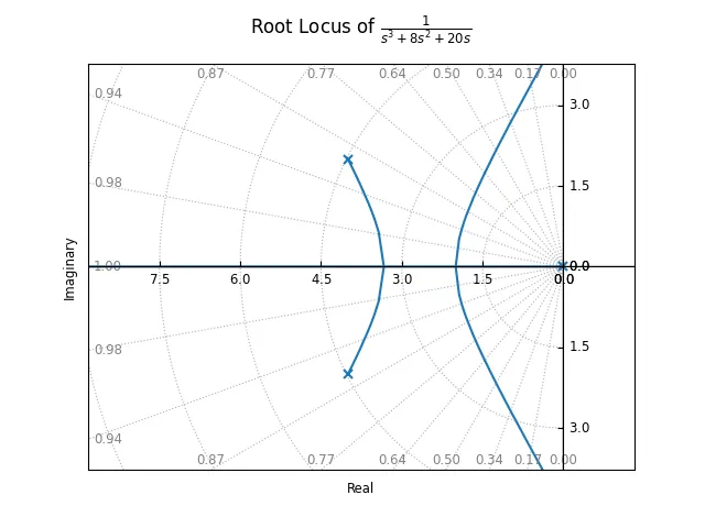
(三)根轨迹
对于开环传递函数为
- 定义函数
1 | # Draw Root Locus |
- 定义传递函数并绘图
1 | # Define Transfer Function |
- 图象
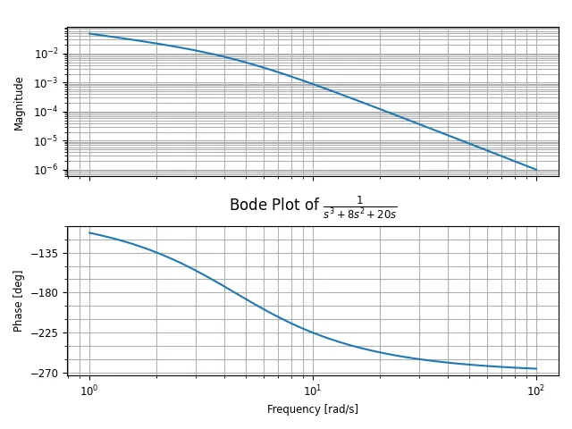
(四)Bode 图
对于开环传递函数为
- 定义函数
1 | # Draw Bode Plot |
- 定义传递函数并绘图
1 | # Define Transfer Function |
- 图象
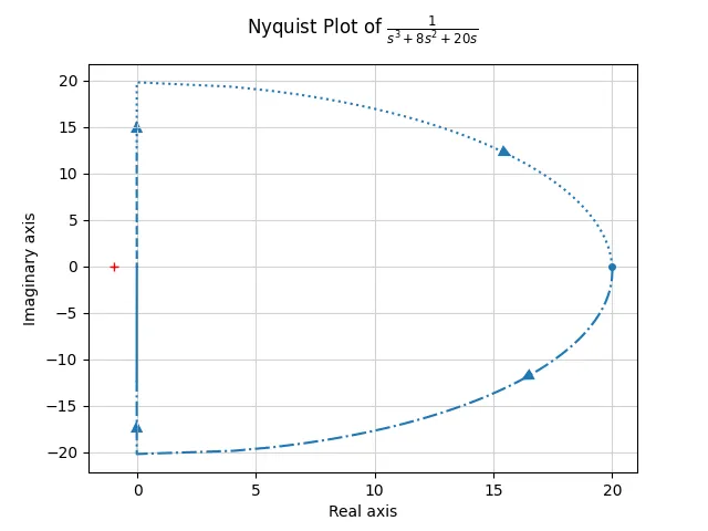
(五)Nyquist 图
对于开环传递函数为
- 定义函数
1 | # Draw Nyquist Plot |
- 定义传递函数并绘图
1 | # Define Transfer Function |
- 图象
三、说明
完整代码见 barkure/py-control。