Barkure

一、前言

我经常需要绘制根轨迹、Nyquist 图之类的图象，MATLAB 启动确实是有点慢，可以使用 Python 的 control 库来迅速的画出所需的图象。

下面是简单的例子。

二、画图

（一）准备工作

1. 安装 control 库：

pip install control

2. 导入所需要的库

下面的库都是后续操作所要使用的：

import control as ctrl
import numpy as np
import matplotlib.pyplot as plt
import sympy as sp
from functools import reduce

3. 定义 tf2latex 函数

tf2latex 用于将传递函数转换成 LaTeX 字符串，方便后续使用。

# Transfer Function 2 LaTex
def tf2latex(sys):
    # Transfer Function to sympy expression
    s = sp.symbols('s')
    num = sp.Poly(sys.num[0][0], s).as_expr()
    den = sp.Poly(sys.den[0][0], s).as_expr()
    sys_expr = num / den
    # sympy expression to LaTex
    sys_latex = sp.latex(sys_expr)
    return sys_latex

（二）系统响应

对于闭环传递函数为 $\Phi(s) = \frac{16}{s^2+10s+16}$ 的系统，绘制其单位冲激响应 $k(t)$ 和 单位阶跃响应 $h(t)$：

1. 定义绘图函数

# Draw Impulse Response
def impulse_response(sys, T):
    title = f'Impulse Response of $' + tf2latex(sys) + '$'
    t, y = ctrl.impulse_response(sys, T)
    plt.plot(t, y)
    plt.title(title, y=1.05)
    plt.xlabel('Time (s)')
    plt.ylabel('Impulse Response')
    plt.grid()
    plt.show()

# Draw Step Response
def step_response(sys, T):
    title = f'Step Response of $' + tf2latex(sys) + '$'
    t, y = ctrl.step_response(sys, T)
    plt.plot(t, y)
    plt.title(title, y=1.05)
    plt.xlabel('Time (s)')
    plt.ylabel('Step Response')
    plt.grid()
    plt.show()

2. 定义传递函数并绘图

# Define Transfer Function
# K, Numerator and Denominator
K = 1

num = [
    [16]
]

den = [
    [1, 10, 16]
]

num[0] = [K * i for i in num[0]]

# Use functools.reduce to automatically calculate the convolution of multiple polynomials
num_conv = reduce(np.convolve, num)
den_conv = reduce(np.convolve, den)
sys = ctrl.TransferFunction(num_conv, den_conv)

# Draw
step_response(sys, np.linspace(0, 5, 1000))
impulse_response(sys, np.linspace(0, 5, 1000))

3. 图象

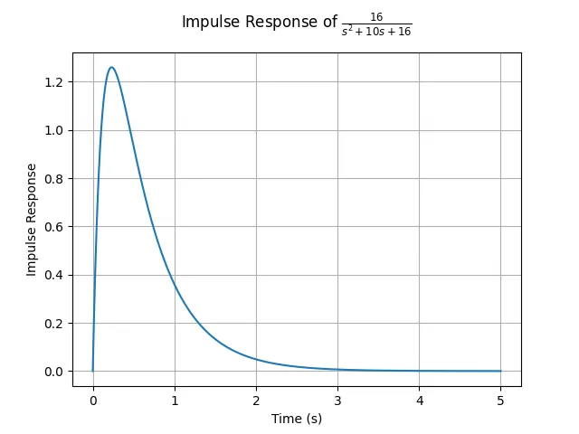
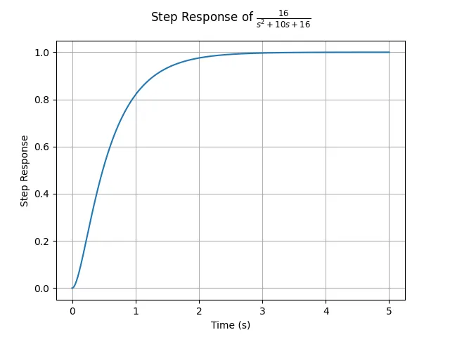
（三）根轨迹

对于开环传递函数为 $G(s)H(s) = \frac{K^*}{s(s^2+8s+20)}$ 的系统，绘制其根轨迹：

1. 定义函数

# Draw Root Locus
def root_locus(sys):
    title = f'Root Locus of $' + tf2latex(sys) + '$'
    ctrl.root_locus(sys, title='')
    plt.title(title, y=1.05)
    plt.show()

2. 定义传递函数并绘图

# Define Transfer Function
# K, Numerator and Denominator
K = 1

num = [
    [1]
]

den = [
    [1, 0],
    [1, 8, 20]
]

num[0] = [K * i for i in num[0]]

# Use functools.reduce to automatically calculate the convolution of multiple polynomials
num_conv = reduce(np.convolve, num)
den_conv = reduce(np.convolve, den)
sys = ctrl.TransferFunction(num_conv, den_conv)

# Draw
root_locus(sys)

3. 图象

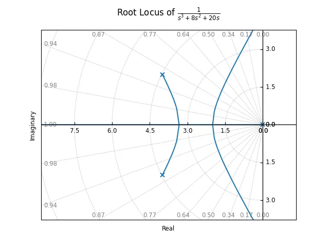
（四）Bode 图

对于开环传递函数为 $G(s)H(s) = \frac{1}{s(s^2+8s+20)}$ 的系统，绘制其 Bode 图：

1. 定义函数

# Draw Bode Plot
def bode_plot(sys):
    title = f'Bode Plot of $' + tf2latex(sys) + '$'
    ctrl.bode_plot(sys, title='')
    plt.title(title, y=1.05)
    plt.show()

2. 定义传递函数并绘图

# Define Transfer Function
# K, Numerator and Denominator
K = 1

num = [
    [1]
]

den = [
    [1, 0],
    [1, 8, 20]
]

num[0] = [K * i for i in num[0]]

# Use functools.reduce to automatically calculate the convolution of multiple polynomials
num_conv = reduce(np.convolve, num)
den_conv = reduce(np.convolve, den)
sys = ctrl.TransferFunction(num_conv, den_conv)

# Draw
bode_plot(sys)

3. 图象

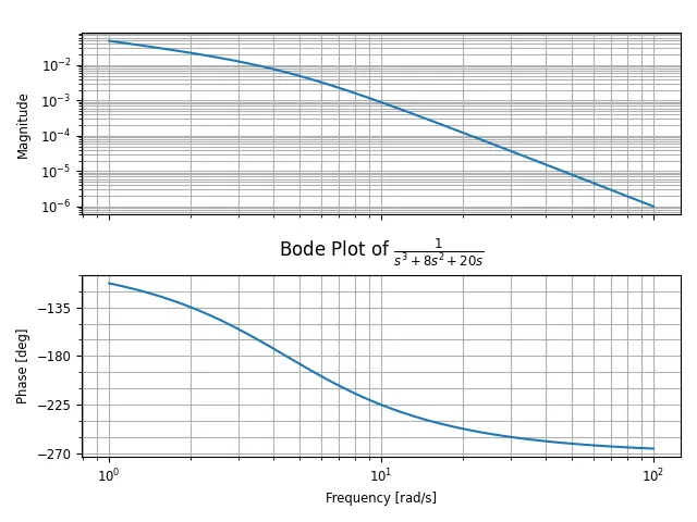
（五）Nyquist 图

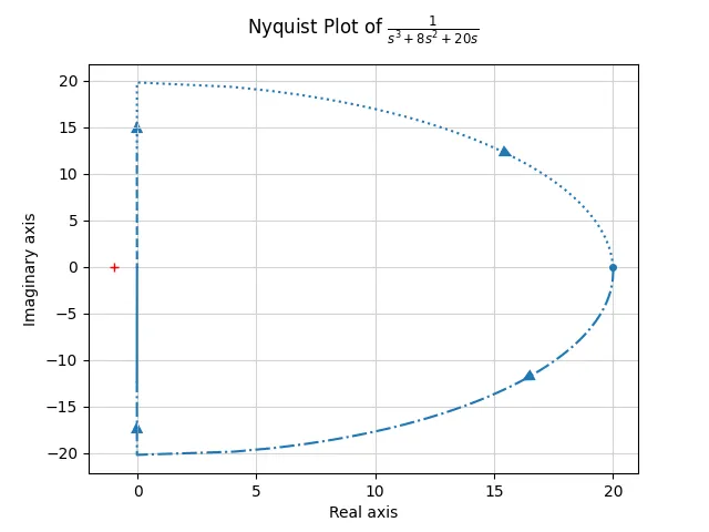
对于开环传递函数为 $G(s)H(s) = \frac{1}{s(s^2+8s+20)}$ 的系统，绘制其 Nyquist 图：

1. 定义函数

# Draw Nyquist Plot
def nyquist_plot(sys):
    title = f'Nyquist Plot of $' + tf2latex(sys) + '$'
    ctrl.nyquist_plot(sys, title='')
    plt.title(title, y=1.05)
    plt.show()

2. 定义传递函数并绘图

# Define Transfer Function
# K, Numerator and Denominator
K = 1

num = [
    [1]
]

den = [
    [1, 0],
    [1, 8, 20]
]

num[0] = [K * i for i in num[0]]

# Use functools.reduce to automatically calculate the convolution of multiple polynomials
num_conv = reduce(np.convolve, num)
den_conv = reduce(np.convolve, den)
sys = ctrl.TransferFunction(num_conv, den_conv)

# Draw
nyquist_plot(sys)

3. 图象

三、说明

完整代码见 barkure/py-control。